How To Draw In Tikz Latex

Part 1 | Part 2 | Part 3 | Part 4 | Part 5

Writer: Josh Cassidy (Baronial 2022)

This five-part series of articles uses a combination of video and textual descriptions to teach the basics of creating LaTeX graphics using TikZ. These tutorials were first published on the original ShareLateX blog site during Baronial 2022; consequently, today'due south editor interface (Overleaf) has changed considerably due to the development of ShareLaTeX and the subsequent merger of ShareLaTeX and Overleaf. Nonetheless, much of the content is still relevant and teaches you lot some basic LaTeX—skills and expertise that will utilize beyond all platforms.

TikZ is a LaTeX packet that allows yous to create high quality diagrams—and often quite complex ones likewise. In this first postal service we'll first with the basics, showing how to describe simple shapes, with subsequent posts introducing some of the interesting things you can do using the tikz bundle.

To become started with TikZ we need to load up the tikz package:

At present whenever we want to create a TikZ diagram nosotros demand to use the tikzpicture surroundings.

                        \brainstorm            {tikzpicture}            <lawmaking goes here>            \cease            {tikzpicture}          

Basic shapes

Ane of the simplest and most commonly used commands in TikZ is the \draw command. To draw a straight line nosotros use this control, then we enter a starting according, followed by two dashes before the ending co-ordinate. We then finish the statement by closing it with a semicolon.

We can then add more than co-ordinates in like this to make it a square:

                        \draw            (0,0) -- (4,0) -- (4,iv) -- (0,4) -- (0,0);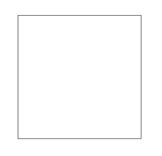          

However this isn't particularly skilful style. Every bit we are drawing a line that ends upwards in the same place we started, information technology is ameliorate to cease the statement with the keyword bike rather than the terminal co-ordinate.

                        \draw            (0,0) -- (iv,0) -- (four,4) -- (0,iv) -- cycle;          

To simplify this code further nosotros can apply the rectangle keyword afterwards the starting co-ordinate and then follow it with the co-ordinate of the corner diagonally opposite.

                        \depict            (0,0) rectangle (four,4);          

We can also add lines that aren't straight. For example, this is how we draw a parabola:

                        \draw            (0,0) parabola (four,4);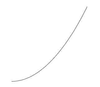          

To add a curved line we use command points. We begin with our starting co-ordinate, then apply two dots followed by the keyword controls and so the co-ordinates of our command points separated by an and. Then subsequently two more dots we have the terminal point. These command points act like magnets attracting the line in their management:

                        \draw            (0,0) .. controls (0,4) and (four,0) .. (iv,4);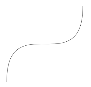          

Nosotros can then add together a circle similar this. The first co-ordinate is the circle's centre and the length in brackets at the stop is the circle'due south radius:

                        \draw            (2,two) circle (3cm);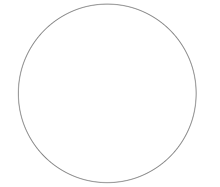          

This is how nosotros describe an ellipse. This time the lengths in the brackets separated by an and, are the x-management radius and the y-direction radius respectively:

                        \depict            (2,two) ellipse (3cm and 1cm);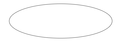          

This is how we draw an arc. In the last bracket we enter the starting angle, the catastrophe bending and the radius. This fourth dimension they are separated by colons:

                        \draw            (iii,0) arc (0:75:3cm);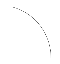          

To customise the way these lines are drawn we add together extra arguments into the \draw control. For example, we can edit the circle we drew so that the line is red, thick and dashed:

                        \draw            [crimson,thick,dashed]            (two,2) circle (3cm);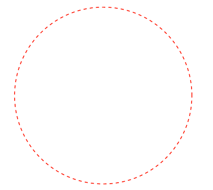          

Grids

Very often when cartoon diagrams we will want to draw a filigree. To practice this we apply the \draw command followed by past some additional arguments. For example, nosotros specify the grid step size using footstep= and a length. We've also specified the colour gray and told it to make the lines very thin. Later these arguments we enter the co-ordinates of the bottom-left corner, followed by the keyword filigree and then the co-ordinates of the top correct-corner:

                        \draw            [pace=1cm,gray,very thin]            (-2,-two) grid (6,6);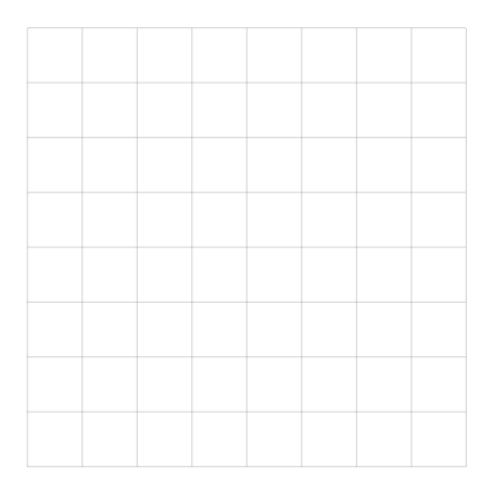          

If nosotros desire to remove the outer lines around this grid nosotros can ingather the size slightly like this:

                        \depict            [step=1cm,gray,very sparse]            (-one.9,-one.9) grid (5.9,five.ix);          

Color filling

At present lets add together a shape onto our grid and color it in. To do this nosotros use the \fill command instead of the \draw command. So in square brackets we enter a colour. For example, this specifies a colour that is 40% blueish mixed with 60% white. Then we just specify a closed shape as we would normally:

                        \fill            [bluish!40!white]            (0,0) rectangle (four,4);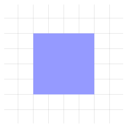          

If we wanted to add a border around this shape we could alter it to the \filldraw control and and so change the arguments so that we take both a fill colour and a draw color specified:

                        \filldraw            [fill up=blue!twoscore!white, draw=black]            (0,0) rectangle (4,4);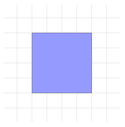          

If instead of one solid colour we want a colour slope, we could change it to the \shade command. Then in the square brackets we specify a left colour and a right colour:

                        \shade            [left color=blue,right color=red]            (0,0) rectangle (4,four);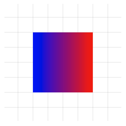          

Instead of doing information technology from left to right we could practise it from top to lesser:

                        \shade            [peak colour=blueish,bottom color=blood-red]            (0,0) rectangle (four,4);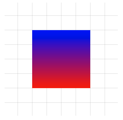          

Or we could even change it by specifying an inner and outer colour similar this:

                        \shade            [inner colour=blue,outer color=crimson]            (0,0) rectangle (4,4);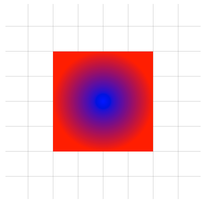          

Finally we could also add together a border to this by using the \shadedraw command and adding a draw colour:

                        \shadedraw            [inner colour=bluish,outer color=red, describe=black]            (0,0) rectangle (4,4);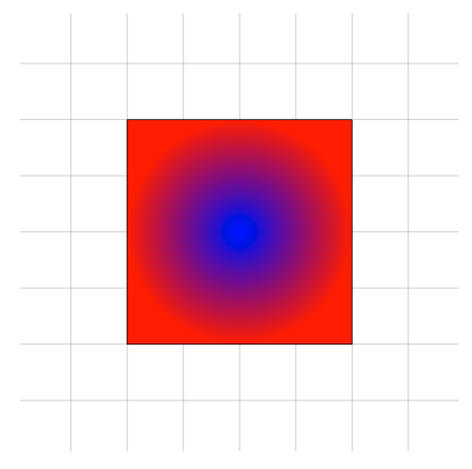          

Axes

Let's finish this post past adding some labeled axes to our grid. To practise this we depict two normal lines both from (0,0), only we'll make them thick and add arrowheads using a dash and a pointed bracket:

                        \draw            [thick,->]            (0,0) -- (4.5,0);            \draw            [thick,->]            (0,0) -- (0,4.v);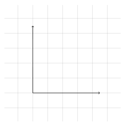          

We can also label our axes using nodes. To exercise this we add the keyword node into both \draw statements next to the end co-ordinates, followed by an anchor specification in square brackets and the text in curly brackets. Every node we create in TikZ has a number of anchors. So when we specify the north west anchor for the ten-centrality node, we are telling TikZ to use the anchor in the top-left-hand corner to ballast the node to the according:

                        \describe            [thick,->]            (0,0) -- (4.5,0) node[anchor=north w]            {10 axis};            \depict            [thick,->]            (0,0) -- (0,iv.5) node[ballast=south due east]            {y axis};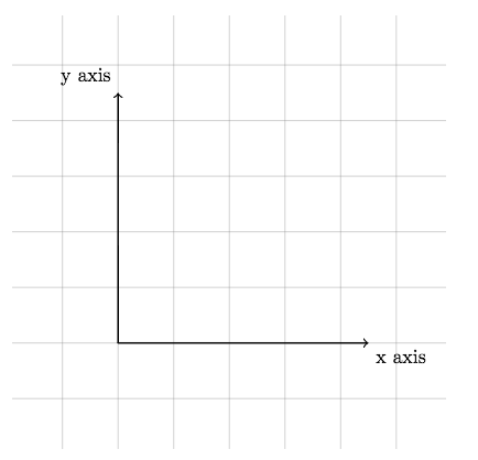          

To finish our axes nosotros tin can add in ticks and numbering like this:

                        \foreach            \ten            in            {0,one,2,3,4}            \describe            (\x            cm,1pt) -- (\x            cm,-1pt) node[anchor=north]            {            $            \x            $            };            \foreach            \y            in            {0,1,ii,3,4}            \draw            (1pt,\y            cm) -- (-1pt,\y            cm) node[anchor=due east]            {            $            \y            $            };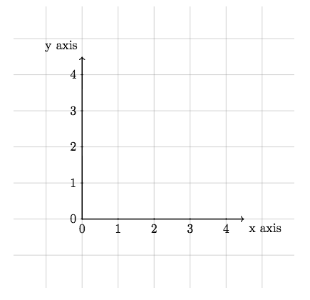          

This clever piece of lawmaking uses two for each loops to systematically go forth the axes calculation the ticks and numbers. In each 1, the variable x or y takes on all of the numbers in the curly brackets, each in plough and executes the \draw control.

This concludes our discussion on basic drawing in TikZ. If you want to play around with the document we created in this postal service you can access it hither. In the side by side post nosotros'll look exporting TikZ code from GeoGebra.

All articles in this series

• Part 1: Basic Drawing;
• Function two: Generating TikZ Code from GeoGebra;
• Part iii: Creating Flowcharts;
• Part iv: Circuit Diagrams Using Circuitikz;
• Office v: Creating Mind Maps.

Please do continue in bear on with us via Facebook, Twitter or via e-mail on our contact usa page.

Source: https://www.overleaf.com/learn/latex/LaTeX_Graphics_using_TikZ:_A_Tutorial_for_Beginners_%28Part_1%29%E2%80%94Basic_Drawing

Posted by: muellerthateadthe.blogspot.com

Share this post